
Cash flow analysis in project finance as it is used in a project finance NPV model to test the debt and equity structure based on the projected cash flows, the interest rate for the financing, and the repayment schedule. Project finance modeling course presents the techniques used to integrate cash flows, debt service and equity into a single model.
What Is a Project Finance NPV Model?
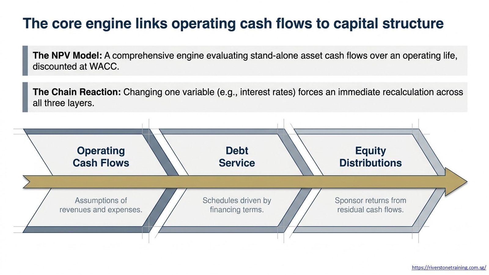
A project finance NPV model is a comprehensive financial model, built in Excel, which is used to project cash flows for a project over its operating life and to discount the cash flows to a present value using the project’s weighted average cost of capital. It is similar to a corporate valuation model, but it is built on a specific asset’s cash flows, with financing on a stand-alone basis, non-recourse or limited-recourse basis.
The operating cash flows are based on assumptions of revenue and expenses, the debt service schedules are based on the structure and terms of the financing, and the equity distributions are based on the return expected by sponsors as the residual cash flows. All three layers are connected in a chain, and one change in an input (e.g., the assumptions for revenue or the interest rate) affects the other two layers.
Why Is Debt and Equity Structuring Critical in Project Finance?
Debt and equity structuring is crucial to making a project financeable, bankable and returns acceptable to its sponsors. In infrastructure projects, the debt-to-equity ratio is a major factor in cash flow split, risk sharing for lenders and investors, and the project IRR, typically 70:30 to 80:20.
A higher debt ratio increases the equity return as a result of leveraging, but also increases the debt service payment, which is what diminishes cash for distributions. The model needs to show that cash flow is available to service the debt in all scenarios and there is no return to equity investors until such cash flow is available. This is the essence of each project finance structuring decision – the leverage efficiency and covenant headroom.
Table 1: Project Finance Capital Structure Components
| Component | Role in Model | Priority in Cash Flow Waterfall |
| Senior Debt | Primary funding, sized against DSCR | First — principal and interest payments |
| Subordinated Debt | Mezzanine layer, higher risk buffer | Second — after senior debt service |
| Equity | Sponsor capital, residual return | Third — distributions after all debt |
| Debt Service Reserve | Liquidity buffer for covenant compliance | Structural — funded before distributions |
| IDC (Int. During Const.) | Capitalised interest in the construction phase | Rolled into total debt at financial close |
How Does a Project Finance Model Link Cash Flows to Capital Structure?
The model connects the cash flows from the business operations to the capital structure using a cash flow waterfall, which is a sequential allocation logic that allocates cash flow in a prioritized manner. Revenue goes into operating costs, and then into debt service (interest and principal), and then into funding of the reserve account, and then into equity distributions. Professionals learning project finance modeling techniques are taught to build this waterfall as a dedicated section of the model, so that every financing decision is traceable to its cash flow impact.
The waterfall arrangement also incorporates covenant logic – such as not allowing equity distributions when the DSCR is below the minimum threshold or the debt service reserve account is not fully funded. This not only enables the waterfall to be used as a financial calculation but also as a built-in covenant compliance mechanism.
How Is Debt Sized in a Project Finance NPV Model?
Debt is sized in a project finance model based on two key limiting constraints: 1. Maximum Debt Service Coverage Ratio (DSCR) and 2. Maximum lenders’ permitted gearing ratio. The model is used to calculate annual debt service (principal and interest) as a function of total debt and then determines if the annual debt service is above the minimum covenant, usually 1.20x to 1.40x by sector.
This puts the model in a circle: debt is used to determine the interest, the interest lowers the project’s free cash flow, and the free cash flow determines the amount of debt the project can bear. The circular reference is resolved by using the iterative calculation feature in Excel or by using a goal seek / macro-based solver. The debt sizing calculation is developed as an independent component that, given the cash flow forecast, lender constraints, etc., generates a maximum debt that the company can assume.
How Do Loan Repayments Affect Project Cash Flow Analysis?
Whichever type of loan repayments are used (equal instalments (annuity), sculpted repayments, or cash sweeps), the free cash flow to be used for equity distributions in each period is reduced. The repayment schedule is represented in a separate amortisation schedule, which determines the outstanding debt balance, the interest expense, and the amount of the principal that is paid off in each of the debt tenor’s periods.
Sculpted debt amortisation, which is often used in infrastructure finance, is one way to adjust repayments to follow the cash flow of the project, such as increasing repayments when cash flows are high and reducing them when cash flows are low due to operating costs. This allows for the maximisation of debt capacity and ensures that the DSCR covenant is not breached throughout the loan tenor. A conditional allocation in the waterfall is used to model cash sweep mechanisms, which accelerate debt repayments when there is excess cash.
Table 2: Debt vs Equity Cash Flow Allocation in the Waterfall
| Cash Flow Level | Allocated To | Modelling Mechanism |
| EBITDA | Operating expenses, taxes | Revenue minus OpEx, then tax calculation |
| CFADS (Cash Flow to Debt Svc) | Senior debt service | EBITDA minus capex and working capital |
| Post-Debt Service Cash Flow | Reserve accounts, sub-debt | CFADS minus total debt service payments |
| Distributable Cash Flow | Equity distributions | Residual after all senior obligations are met |
| Cash Sweep (optional) | Accelerated debt repayment | Conditional — triggered by excess cash |
How Is Equity Return Calculated in Project Finance Models?
The return to equity is the main measure of a project finance model, and is measured by the Equity IRR, which is the internal rate of return on the equity invested, determined by discounting equity cash flows (investments at construction time and distributions at operations time) back to the time of first equity investment. The equity multiple is a secondary measure; it is a multiple of the equity invested and is the total amount of distributions received.
The equity cash flow is an output of the waterfall: equity cash flows are negative during construction and equity cash flows (post-debt-service free cash flow) are positive during operations. This equity cash flow series is used as input for the Excel function: =XIRR. This function calculates an annualised return based on the real dates.
How Does the Model Reflect Interest During Construction (IDC)?
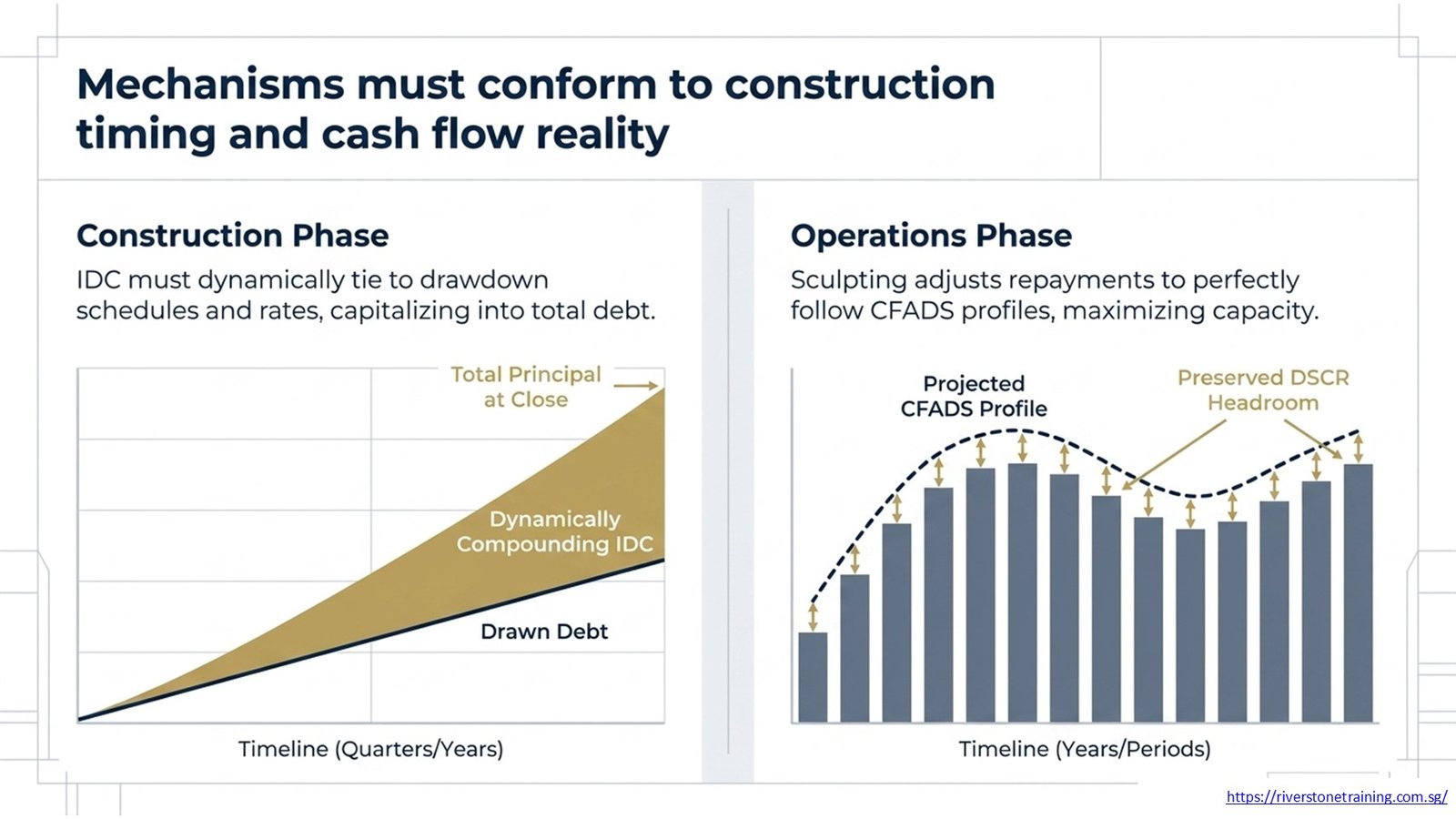
Interest During Construction (IDC) is the interest on the drawn debt while the construction process is ongoing and the project has not yet started generating income. The total debt amount, in most project finance structures, is capitalised (financed in as opposed to paid in cash) and, therefore, is greater than the amount of the initial funding by the total amount of interest accrued.
The model should be dynamic and should enable calculation of IDC according to the debt drawdown schedule, the prevailing interest rate, and the construction period. One common error is assuming a fixed IDC amount instead of tying the amount to the balance drawn and the assumptions of the rate. If IDC is modeled properly, then when rates or construction time changes, total debt automatically updates and consequently so do the DSCR calculations and equity returns.
How Do DSCR Constraints Influence Debt Structure?
The Debt Service Coverage Ratio (DSCR) is the most important credit measurement that lenders will use to determine project feasibility and size the debt. It is the ratio of Cash Flow Available for Debt Service (CFADS to total debt service, measured for each period. Lenders have a minimum DSCR covenant (typically 1.20x for operating infrastructure) that the model must demonstrate throughout all operating periods and scenario cases.
If DSCR is lower than the minimum in the model, it indicates that debt is excessive in comparison to cash flows. The analyst has to then either reduce the total debt, restructure the repayment schedule, or have to change the project assumptions. The DSCR constraint is not merely a covenant check, but a prime enabler of debt quantum, debt tenor and amortisation profile for each project finance structure.
Table 3: NPV vs IRR — Interpretation in Project Finance
| Metric | What It Measures | How It Guides Decisions |
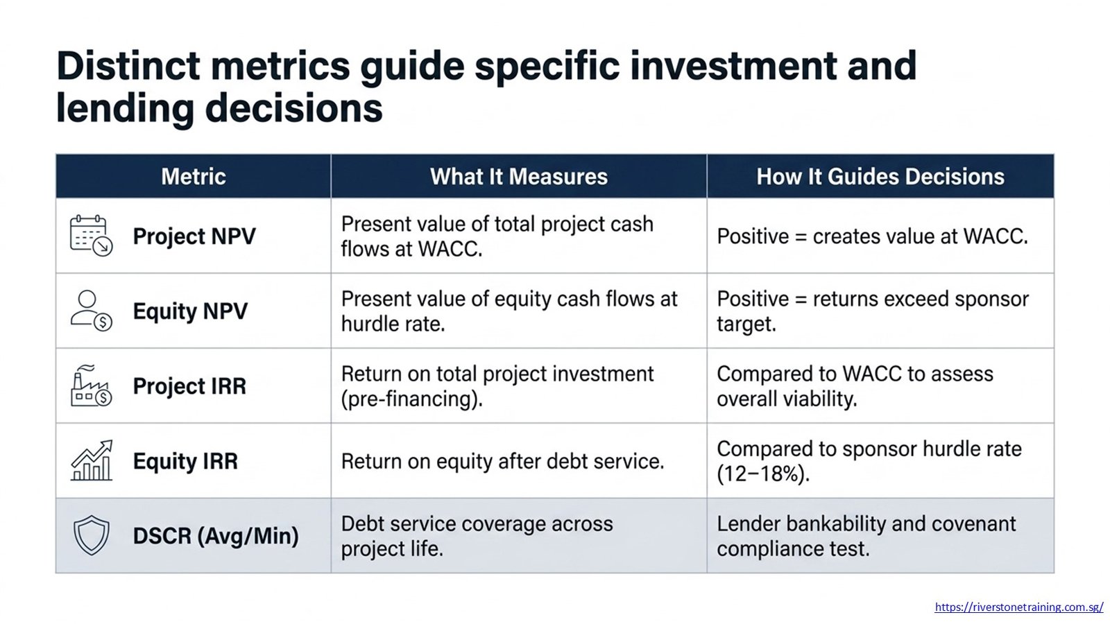
| Project NPV | Present value of total project cash flows at WACC | Positive NPV = project creates value at WACC |
| Equity NPV | Present value of equity cash flows at the hurdle rate | Positive equity NPV = returns exceed sponsor target |
| Project IRR | Return on total project investment (pre-financing) | Compared to WACC to assess overall viability |
| Equity IRR | Return on equity investment after debt service | Compared to sponsor hurdle rate (e.g., 12–18%) |
| DSCR (avg/min) | Debt service coverage across the project life | Lender bankability and covenant compliance test |
How Does WACC Impact Project Finance NPV Calculations?
In project finance, WACC is the weighted average of the cost of debt (after tax) and the required return on equity, with the proportions that they make up of the total project capital. Used to discount the project NPV calculation and it is the lowest return the project should return to meet the expectations of all capital providers. If the NPV of a project exceeds the zero value at WACC, then it is value accretive.
Any changes in the debt-equity ratio will have an immediate impact on WACC. The more leverage employed, the lower WACC will be (as debt becomes cheaper than equity, on a post-tax basis); but, the higher the risk and required return on equity. The model should be set up so that the WACC is recalculated when the financing structure changes — if the capital structure is optimised in an iterative manner, the NPV results will be misleading if the WACC is assumed to be static.
How Is Equity IRR Derived From Project Cash Flows?
The equity cash flow series is used to calculate the equity IRR, and the model calculates it from the equity contributions removed from the funding schedule in the construction period and the equity distributions in the operating period from the waterfall. The difference between the two is always positive, as leverage is positive and represents the value of financial leverage for equity investors; equity IRR is always greater than Project IRR.
An average IRR (real or nominal, depending on the contract) for infrastructure equity is 10-15%. If the Equity IRR is under this threshold, analysts consider such options as increasing leverage, renegotiating offtake contract terms, or reducing the construction costs to improve returns. Sponsors can consider reducing tariff assumptions to lower equity returns as bids to achieve acceptable returns on equity, while maintaining project viability, particularly if the equity IRR is outside of the acceptable range.
How Do Scenario and Sensitivity Analysis Test Financing Structures?
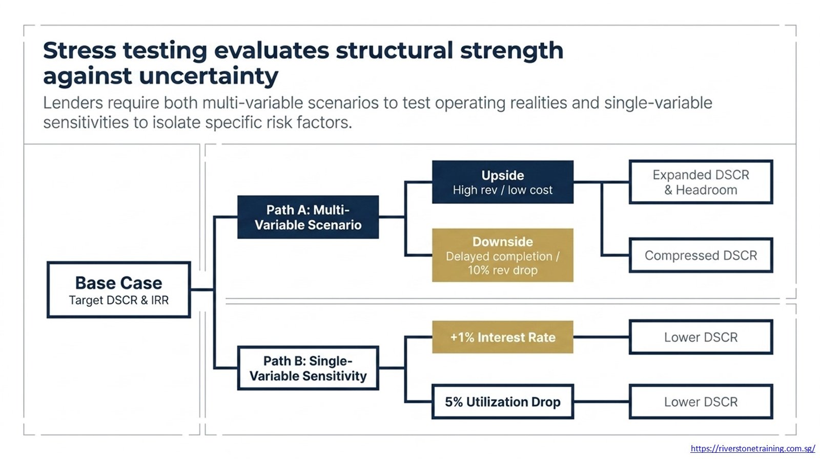
A scenario analysis assesses if the financing structure will be viable given a number of potential operating scenarios, such as a 10% reduction in revenues, a construction completion delay, or an ongoing rise in operating expenses. A good project finance model consists of at least three scenarios (base, upside, downside) and should also include different levels of DSCR, NPV, and Equity IRR for each scenario to evaluate the strength of the financing structure. This is a core skill covered in any serious project finance modeling course curriculum.
Sensitivity analysis tends to be at the level of a single variable; it shows the effect of any single sensitivity change, e.g. a 1% rise in interest rates or a 5% drop in utilisation, on the major outputs. The most common tool is a sensitivity table (data table in EXCEL) which creates a table of DSCR or IRR results for a variety of combinations of assumptions. Most lenders will request both a scenario and a sensitivity analysis when considering a loan application.
Table 4: Financing Constraint Impact on Capital Structure
| Constraint | Effect on Debt Structure | Model Adjustment Required |
| Minimum DSCR (1.20x) | Limits the maximum debt quantum | Reduce debt or sculpt amortisation |
| Maximum Gearing (80%) | Caps debt as % of total project cost | Increase equity contribution |
| Minimum LLCR | Tests debt over the full loan life | Extend tenor or reduce drawings |
| Interest Rate Increase | Increases debt service, reduces DSCR | Re-size debt, adjust repayments |
| Construction Overrun | Increases total debt (IDC and cost) | Contingency reserve, cost review |
| Target Equity IRR | Drives minimum equity leverage required | Optimise debt/equity ratio |
What Trade-Offs Exist Between Debt Leverage and Equity Returns?
The positive leverage effect occurs when the project return is greater than the cost of debt; higher leverage shows up in higher Equity IRR. It also raises the debt service coverage ratio (DSCR) needed to meet the debt obligations, creates DSCR headroom constraints and further constrains equity cushions to cushion downside scenarios. The model also shows the impact of these levers on Equity IRR, minimum DSCR, and equity NPV, making these trade-offs explicit.
At a certain cut, so does the benefit of the return of the loan exceed the financial risk — and lenders will refuse to lend or require a higher interest margin to cover the extra risk. It is the margin at which the minimum DSCR in the downside scenario dips below the lender covenant – determined by the analysts – and this is considered the actual leverage cap.
What Common Mistakes Do Analysts Make in Project Finance NPV Modeling?
The most frequently made mistake that people make when modelling is to consider IDC as a fixed number instead of a variable number that is related to the drawdown schedule and the interest rate. This results in an inaccurate total debt balance and doesn’t reflect the cost and DSCR impact of construction delays or escalation. A related mistake is using a constant WACC for the NPV analysis without adjusting it for changing debt/equity ratios in scenario analysis.
Common errors include simple equal installment amortisation that does not incorporate the cash flow profile in the actual debt size, as well as not performing the circularity check that will ensure the debt size and DSCR converge on an iterative basis. These errors can be avoided using a structured approach to model building, as taught in a systematic finance modelling course.
How Do Lenders Use NPV Models to Evaluate Risk?
The NPV model (and the DSCR profile it generates) is applied to determine if project cash flows have enough headroom and can cover debt payments over all periods and scenarios. They emphasize minimum DSCR as well as the Loan Life Coverage Ratio (LLCR) and break-even revenue level, which are important measures of credit risk, throughout the life of the loan.
When submitting the sponsor’s model to the credit committee, lenders normally ask for the sponsor’s financial advisors to have the model reviewed independently by their financial advisors, who then reconstruct or stress test the model using downside assumptions. Knowing how to use the model is thus as significant as knowing how to construct the model, and the best project finance modeling techniques training programmes incorporate this knowledge into their training.
Table 5: Project Finance NPV Modeling Workflow
| Step | Model Activity | Key Output |
| 1 | Create a forecast of build revenue and operating costs. | EBITDA and CFADS by period |
| 2 | Structure construction cost and drawdown schedule | Equity and debt contributions by phase |
| 3 | Calculate IDC and total debt at financial close | Debt balance and capitalised interest |
| 4 | Size senior debt using DSCR and gearing constraints | Maximum debt quantum and amortisation |
| 5 | Build a debt service schedule and an amortisation table | Interest, principal, and outstanding balance |
| 6 | Create a cash flow waterfall chart. | Distributable cash flow, equity returns. |
| 7 | Compute Project IRR, Equity IRR, NPV, DSCR | Investment decision metrics |
| 8 | Run scenario and sensitivity analysis | Downside DSCR, IRR range, covenant headroom |
Conclusion
The project finance NPV model isn’t just a valuation model; it is an engine for structuring a financing decision. Analysts can use the model to simulate different operating cash flows, debt service schedules, reserve accounts and equity distributions to determine if a specific capital structure is bankable, viable and will deliver the desired return to all parties. All of the elements of the model, such as IDC calculations and DSCR covenant checks, are a direct reflection of the terms being negotiated in the real world between sponsors, lenders and offtake counterparties.
Debt and equity structure in project finance models is a complex exercise that requires a detailed understanding of the interdependencies of each modelling decision to master the debt and equity structure. Understanding how to eliminate circularity in debt sizing, design sculpted amortisation schedules and stress test structures under downside scenarios can be used in real infrastructure and energy transactions and offers a level of technical fluency that is relevant to actual work. In the world of project finance, infrastructure advisory, and development banking, a structured project finance modeling course offers a structured pathway towards becoming a skilled and credible, commercially viable finance professional.